Closed-loop evaluation modes

python/vdsim_closedloop.py runs one controller callback against a VDSimPlant under three timing models, so the cost of controller computation delay and loop jitter can be measured with everything else held equal. The controller does not change between modes; only the mode string does.

from vdsim_closedloop import ClosedLoopEval, LatencyModel

def controller(obs, t):            # obs: VDSimPlant observation dict at time t
    return delta_rad, fx_total_n

ev = ClosedLoopEval(
    plant_kwargs=dict(level="L2", substep_dt=5e-4),
    controller=controller,
    control_period=0.02,           # Tc [s], a whole multiple of substep_dt
    mode="virtual_async",          # "sync" | "virtual_async" | "wallclock"
    latency=LatencyModel.fixed(0.010),
    overrun="skip",                # "skip" | "queue"
    duration=10.0,
    trace_path="runs/b10.vdtrace", # optional .vdtrace
    reference_path=path_xy,        # optional (M, 2) polyline -> e_y stats
)
res = ev.run()                     # res.trace, res.samples, res.stats, res.meta

Which mode to use

Mode	Clock	Delay in the loop	Reproducible	Use it for
A sync	virtual, one thread	none: command applied at its sample time	bit for bit	the reference result; identical to a VDSimPlant.step loop
B virtual_async	virtual, one thread	c_k from a LatencyModel, inserted in virtual time	bit for bit for fixed and seeded distributions	sweeping a delay budget; regression tests of delay sensitivity
C wallclock	wall clock, C++ sim thread + Python control thread	whatever the host really took, OS jitter included	statistically only	checking that a controller keeps up in real time on a given host

A sync

At t_k = k*Tc the observation is sampled, the controller is called and its command is applied at once and held for one period (zero-order hold). The result is bit-identical to the documented VDSimPlant loop.

B virtual_async

The sample at t_k produces a command that takes effect at

t_apply = ceil((t_k + c_k) / substep_dt) * substep_dt

The previous command stays in force until then; the plant keeps integrating substep by substep. One worker computes one sample at a time: sample k starts at max(t_k, finish of k-1).

When a computation runs past the next grid point (c_k > Tc) the run is in overrun and the overrun policy decides:

• skip: samples that fall due while the worker is busy are not taken; the next sample is the first grid point at or after the finish.
• queue: every grid sample is taken at its own time and computed in order, so the delay accumulates while c_k > Tc.

Both count overruns in stats["n_overrun"]; skip also counts stats["n_skipped"].

Latency models:

Model	c_k	Reproducible
LatencyModel.fixed(c)	c every sample	yes
LatencyModel.uniform(lo, hi, seed)	U[lo, hi] from a generator seeded per run	yes, per seed
LatencyModel.normal(mu, sd, seed)	max(0, N(mu, sd^2)), clipped at zero because a computation cannot finish before it starts	yes, per seed
LatencyModel.measured()	wall time of the controller call (time.perf_counter)	no

fixed(0) reproduces mode A bit for bit for both policies.

C wallclock

A C++ vdsim.RealTimeRunner ticks the session every substep_dt of wall clock with Python's global interpreter lock (GIL) released. A Python thread wakes every Tc, snapshots the session, calls the controller and latches its command through the same Fx -> wheel torque mapping that VDSimPlant uses. The controller may block or spin; the sim keeps advancing (the delay is real, not modelled).

stats reports the control period p50/p99/max (median, 99^th percentile, maximum), the wake jitter, the sample-to-apply delay, overruns, skipped slots and the real-time factor rtf = elapsed virtual time / elapsed wall time (closer to 1 is better). ev.stop() ends a run early from any thread; every exit path (normal end, controller exception, stop(), KeyboardInterrupt) joins both threads before run() returns.

Options that exist only in this mode:

• cpu_affinity={"sim": 2, "ctrl": [3]} pins the sim thread to one core and the control thread to a core set. Linux only (sched_setaffinity); on other platforms the request is ignored and stats["sim_affinity_applied"] / stats["ctrl_affinity_applied"] say so. The default (None) inherits the process affinity, so taskset around the process decides.
• watchdog={"timeout_s": 0.1, "failsafe_u": (0.0, -2000.0)} latches a fail-safe command whenever no command arrived for timeout_s; latches are counted in stats["failsafe_latches"].

What each mode does not promise

• A and B do not measure your controller's speed; B uses the delay you give it (or, with measured(), a single host's timing without OS scheduling).
• C is not reproducible. Two runs differ; compare distributions, not runs.
• C jitter depends on the host load and the OS scheduler. VDSim does not provide real-time kernel guarantees. The numbers below are what one shared Linux host gave, not a bound.
• Core pinning is Linux-only (see above).
• A queued sample in C is the state when the control thread gets to it, not the state at its slot: a real-time loop cannot read the past.

Results and trace

• res.trace: arrays per control sample (t, pose and velocities, u_steer/u_fx = command in force at that instant; u_ax in place of u_fx with longitudinal="accel"). A and B are on the grid t_k = k*Tc plus a closing row at duration without a command; C has one row per wall-clock sample (irregular t).
• res.samples: one row per controller sample actually taken: k, t_sample, t_apply, c_k, overrun, applied, the command, and the measured compute time t_compute_s.
• res.meta: eval_mode, control_period_s, latency_model, overrun_policy, delta_sw_ratio, level and (C) affinity and watchdog; the provenance of Using VDSim from another repository; longitudinal / accel_conversion (Acceleration command); ref_point and tracking_point (Reference point).
• trace_path= writes a .vdtrace (schema 0.5) with one row per control sample. A writes exactly what VDSimPlant.enable_trace writes. B and C add four channels that describe the command in force on that row:

Channel	Unit	Meaning
t_sample	s	virtual time at which that command's observation was sampled
t_apply	s	virtual time at which it took effect
c_k	s	its computation delay (B: the latency model; C: measured)
overrun	-	1 when its computation ran past one control period

The rows before the first computed command carry NaN times and overrun = 0. The manifest records eval_mode, control_period_s, latency_model and overrun_policy in every mode. The four channels are optional and additive, so the schema stays 0.5 and an existing 0.5 reader ignores them.

Ending a run early

ev.stop() ends a run in every mode. Call it from the controller or from any other thread; run() then returns what ran so far.

Mode	Where the run ends	The command of the stopping call
A sync	a stop() made while a controller call runs: at that sample's time t_k; a stop() made between calls: at the next grid time, before that sample is taken	not applied; the plant is not advanced
B virtual_async	as in A, at the virtual time of the call. A queue sample computed late behind a busy worker is called at the substep the worker frees up, so the run ends there (the plant cannot go back to t_k)	not applied; every command still waiting for its t_apply is dropped too
C wallclock	the control thread stops at its next slot and the sim thread is joined; the run ends wherever the session clock got to	unchanged from before

• stats["stopped_early"] (bool) and stats["t_stop"] (simulated end time [s], None when the run went the full duration) are present in every mode. meta["duration_s"] stays the nominal duration; the run's real length is t_stop.
• Dropped commands are counted in stats["n_unapplied"] with applied = 0 in res.samples; they never appear as a t_apply in the trace.
• res.trace ends with a closing row at t_stop (no command), and the tracking metrics of reference_path use only the samples that ran.
• A recorded trace is finalized normally: its last row is t_stop (when that row falls on the decimation grid; at Tc >= 10 ms it always does) and the manifest carries stopped_early and t_stop. A run that is not stopped records stopped_early: false, t_stop: null.
• stop() before run() has no effect: every run starts cleared.

Realized steer

The observation carries the steer the dynamics actually integrated, after the actuator chain (dead time, lag, rate limit) of actuator=:

Key	Unit	Meaning
delta_rw	rad	realized road-wheel steer over the last substep before the sample. With actuator=None it equals the command in force, bit for bit
delta_sw	rad	delta_rw x steering_ratio, only when the vehicle file states steering_ratio; no default ratio stands in for it. The ratio used is meta["delta_sw_ratio"] (None = not observed)

res.trace has a delta_rw column. trace_channels=("steer_applied",) adds the same quantity to the .vdtrace as an optional channel (rad); it is off by default so the default trace is unchanged, and a 0.5 reader that predates it ignores it. Per-wheel steer angles are not observed: the direct-control plant applies one road-wheel angle.

Yaw acceleration r_dot is not provided: the dynamics' derivative cannot be read out without a core interface change, and a finite difference of r is not offered in its place.

Reference point

ref_point= (a VDSimPlant argument, so it also goes in plant_kwargs) adds the motion of one body point to every observation. X, Y stay at the CG.

Value	Point (body frame, ISO 8855: x forward, y left)
None (default)	nothing added
"cg"	[0, 0]
"rear_axle"	[-cg_to_rear, 0]
"front_axle"	[cg_to_front, 0]
[x_fwd, y_left]	that offset [m]

Key	Unit	Meaning
X_ref, Y_ref	m	ground position of the point
vx_ref, vy_ref	m/s	its velocity in the body frame, v_P = v_CG + r x p: vx - r*y_left, vy + r*x_fwd

meta["ref_point"] and the trace manifest record the setting, the offset used and cg_to_front_m / cg_to_rear_m. The tracking error of reference_path is still measured at the CG (meta["tracking_point"] = "cg").

Acceleration command

With longitudinal="accel" the second command element is a longitudinal acceleration target [m/s^2] instead of a force [N]:

ev = ClosedLoopEval(dict(config="generic_sedan.yaml", longitudinal="accel"),
                    controller,           # returns (delta_rad, ax_mps2)
                    control_period=0.02)

• One converter: the session's L5 cascade, LongAxController (PI plus feed-forward on the measured ax), the class and gains the RL accel action uses. Its pedal output becomes wheel torque linearly: throttle x drive_torque_ref and brake x brake_torque_ref, split with the vehicle's front share. Non-positive references fall back to max_motor_torque x final_drive_ratio and max_brake_torque.
• No resistance or mass feed-forward is added; the integrator absorbs the steady drag and rolling resistance. The target is not clamped; full pedal is the ceiling.
• Not the RL accel response: the RL environment's pedals drive the vehicle's powertrain map, while here they scale the linear torque references above.
• meta["accel_conversion"] (and the trace manifest) records the converter, its gains, both references and these choices. In force mode it is None and the manifest has neither key.
• The target is recorded as u_ax [m/s^2] in res.trace, res.samples and the trace file; u_fx is absent from all three in accel mode, so a reader that takes u_fx as a force [N] never sees an acceleration. A schema 0.5 reader that predates u_ax opens such a trace and ignores the channel.
• L1 is refused: the bicycle model reports ax = 0, so the feedback has nothing to track.

Using VDSim from another repository

Pin a commit, build the bindings and install the Python layer in editable mode:

git clone https://github.com/Onlyti/VDSim.git && cd VDSim
git checkout <sha>
pip install -e .            # builds the bindings (scikit-build-core)
python -c "import vdsim; print(vdsim.__version__, vdsim.__git_sha__, vdsim.__git_dirty__)"

The build bakes the source HEAD into the module: vdsim.__git_sha__ (40 hex digits, "unknown" without git at build time) and vdsim.__git_dirty__ (True when tracked files differed from HEAD, None when unknown). Every result carries it, so a stored result says what it ran on:

res = ev.run()
assert res.meta["vdsim_git_sha"] == "<sha>"
res.meta["vdsim_version"], res.meta["param_hash"], res.meta["vehicle_config"]
res.meta["level"], res.meta["actuator"]   # None, {"preset": id} or {"param_hash": ...}

The same functions fill the trace repro block. Tagged releases and PyPI packages are not published for this yet; pin by SHA.

Example: delay budget of a lane-change controller

examples/closed_loop_eval_demo.py runs a Stanley-type lateral controller with a speed loop on a double lane change (3.5 m over 30 m, 20 m/s, L2, Tc = 20 ms, substep_dt = 0.5 ms) as A, B with fixed delays of 0, 5, 10 and 20 ms, and C five times.

Metric: e_y = signed distance [m] from the CG to the closest point of the reference polyline, along its normal, ground frame (vdsim_closedloop.lateral_error); RMSE over every control sample (lower is better). C is the mean ± standard deviation of five runs.

taskset -c 0-9,12-23 python3 examples/closed_loop_eval_demo.py --out demo_out

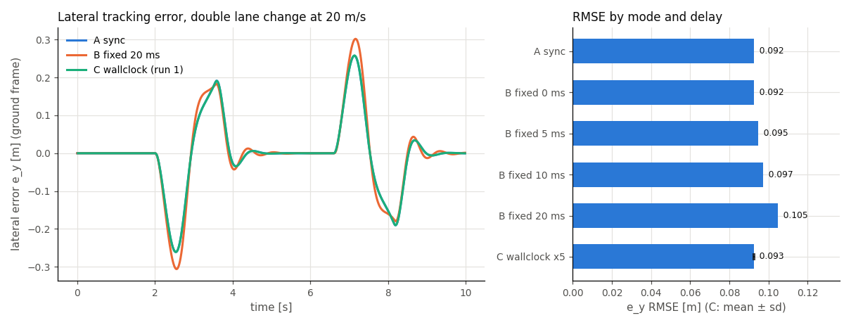
case	e_y RMSE [m]	max abs e_y [m]	samples	overruns
A sync	0.0924	0.2609	500	0
B fixed 0 ms	0.0924	0.2609	500	0
B fixed 5 ms	0.0946	0.2710	500	0
B fixed 10 ms	0.0972	0.2818	500	0
B fixed 20 ms	0.1048	0.3059	500	0
C wallclock x5	0.0927 ± 0.0003	0.2634	500 (mean)	0 (total)

Mode C ran with load1 = 16.7 on cores 0-9,12-23 (inherited); its sample-to-apply delay p50 was 0.1 ms and its period p99 at most 28.6 ms.

B shows how the same controller loses tracking as its computation delay grows (B 0 ms equals A exactly). C stays close to A because this controller computes in well under a millisecond, so its real sample-to-apply delay is a fraction of a substep.

Wall-clock jitter measured on a shared host

One Linux host (24 logical cores, cores 10 and 11 excluded with taskset), L2, Tc = 20 ms, substep_dt = 0.5 ms, 10 s runs, cheap controller. load1 is the one-minute load average read just before the run. Control period = time between consecutive wakes of the control thread; overrun = latch later than one period after its slot.

Condition	load1	Cores	Runs	Period p50 [ms]	Period p99 [ms]	Period max [ms]	Overruns per run (of 500)	RTF
low load	2.86–3.90	inherited 0-9,12-23	5	20.00	20.05–20.07	20.06–20.12	0/0/0/0/0	0.99999
shared-host load	~17	inherited 0-9,12-23	5	20.00	22.67–28.68	29.41–34.80	0/0/0/0/0	0.99947–0.99999
shared-host load	~17	pinned: sim core 2, control core 3	5	20.00	25.55–33.49	30.79–45.28	2/4/0/3/0	0.99999
shared-host load	~17	pinned: sim core 15, control core 13	3	20.00	20.44–30.01	30.26–40.09	1/0/0	0.99879–0.99999

All runs on 2026-10-13 with examples/closedloop_wallclock_bench.py and the S6 test; RTF is given to five decimals.

Under heavy load the period p99 spreads to roughly 20-34 ms while the RTF stays near 1; at low load it stays within about 0.1 ms of Tc.

Limits observed under load

The wall-clock pass lines (S6 RTF band, S7 "sim keeps ticking while the controller blocks") are registered as the ctest closedloop_wallclock_timing with the label timing. The validation preset and the CI build jobs exclude that label because a shared CI runner's load is not under our control; the verdicts are measured locally at low load instead.

S7 asserts that at least 96 of the nominal 120 sim ticks (0.8 x 120) happen while the controller blocks for 3*Tc. Observed failure rates:

Condition	load1	Runs	Runs below 96 ticks	Fewest ticks
low load, 4 variants (sleep / GIL-holding spin x skip / queue) x 20	3.13–3.97	80	0	120
shared-host load, standalone	13.8–18.7	80	0	104
shared-host load, right after a 10 s S6 run	16.3–20.6	40	1	86
shared-host load, inside a full ctest run	~18–20	2 suite runs	2	82

On a heavily loaded host expect occasional misses of the tick floor; measure mode C on a quiet machine or treat its numbers as host-specific.

Each wallclock result carries flags to filter on:

• stats["load1_start"]: 1-minute load average just before the run (Linux; None elsewhere).
• stats["rtf_windows"]: RTF per 1 s of wall clock, p01 / p50 / p99 / min and the window count n (None under two windows).
• stats["quality"] = {"ok": bool, "reasons": [...], "warnings": [...]} with fixed rules: "rtf_band" when |rtf - 1| > 0.02, "sim_max_lag" when sim_max_lag_s > Tc, "sim_ticks_short" when a run that was not stopped took fewer substeps than planned.
• ok answers "can the measuring environment (the sim thread) be trusted"; warnings answers "did the controller miss its period". The only warning is "control_overrun" (n_overrun > 0); it never changes ok, because a slow controller is the result being measured, not a broken environment.

runs = [ev.run() for _ in range(5)]
kept = [r for r in runs if r.stats["quality"]["ok"]]          # trusted runs
on_time = [r for r in kept
           if "control_overrun" not in r.stats["quality"]["warnings"]]

Contention on the controller side adds delay too: an inference library whose thread count is not fixed can compete with the sim thread for cores.